Lecture 3
Basic
- Overview of CNNs
- A special case of MLP
- Commonly apply to visual object or 2D array input
- Unified feature extractor and classifier in one network
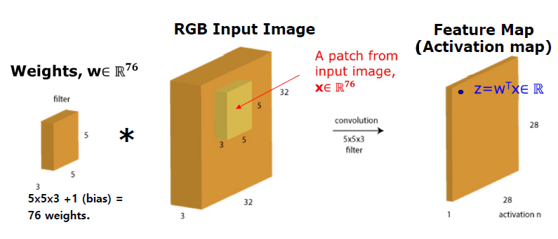
- Filter kernel = weights in between layers
- Feature map = filtered outputs
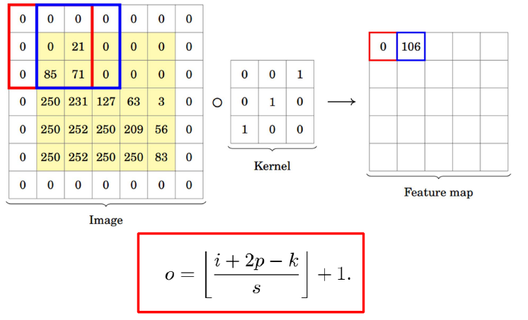
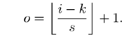
How can compute Feature Map Size?

i = input size, k = filter size(kernel), s = stride, o = output feature map size
if o<i, can occur some problem
then, we can use Zero Padding
At same points, we can apply multiple filters. We call it "channel"
Two Characteristics of CNNs
- Local Connectivity - image is locally correlated
- Weight Sharing- overcome enormous weights problem
Local Connectivity
- MLP : Weights are fully connected, ie. MLP use all weights
- CNNs : One neuron will connect to filter size chunk , thus only have 5x5x3 weights
Receptive Field(RF)
How much a convolution window "see" on it's input image or part of the image that is visible to one filter at a time
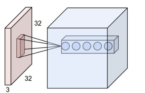
In upper figure, dark pink square in left light pink square(32x32x3) is Receptive Filed.
It means "Receptive Filed size == filter size"
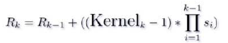
- How the later feature map "see" the image?
Weight Sharing
- MLP has different weights for every single neuron.
- Total # of weights = (filter size) x (Input_w x Input_h x # of feature maps) = too many!
- CNN has same weight for every single feature map
- Total # of weights = (filter size) x # of feature maps = small than MLP
Max Pooling
Pooling does resize the activation map from convolution to get new layer.
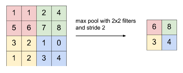
- Output size (o)
- Input size (i)
- Pooling window size (k)
- Stride (s)
Fully Connected (FC) layer
- FC layer started right after the last convolution or pooling layer
- Flatten pooling layer = input layer of MLP
- Last FC layer = output layer of ConvNet. It uses several tasks like classification.
Summary
Typical ConvNet process : [CONV layer - ReLU-Pooling] x N - [FC-ReLU] x M - FC - (softmax or sigmoid)
Parameter in CNN
- Conv layer
- Filter window size (Odd number)
- Number of Filters (Power of 2)
- Stride
- # of Conv layers
- Pooling layer
- Pooling window size
- stride
- # of pooling layer
- Fc layer
- # of hidden nodes
- # of FC layer
- BP algorithm
- Learning rate, batch number, momentum coefficient, L2 coefficient
Feature Normalization in CNN
Batch Normalization(BN)
- Using mean and variance of each feature, Normalize each feature in batch
- normalize feature map of each channel over a batch sample
Layer Normalization(LN)
- Using mean and variance of each feature in input, normalize each input in batch
- applicable to dynamic network and recurrent network(good)
- normalize entire feature map

Instance Normalization
- It is similar with LN but not applicable to MLP and RNN. It is best for CNNs.
- Effective for style transfer and image generation tasks using GAN
- Compute mean and variance each sample in each channel
Group Normalization
- It is similar with Instance Normalization but not applicable to MLP and RNN. It is best for CNNs.
- Effective for object detection, video classification (It is effective in memory problem)
- Compute mean and variance each sample in each group that channels are grouped by group size g.
- In image, The center of image and edge of image do not have equal meaning.
- Thus, We can get flexibility if we compute differently each channels.
- Also, Image's channel is not independent. If we use some channels nearby pivot channel, we can apply normalization at large region.
- Conv layer
Storage and Computational Complexity
- ci-1 = previous layer channel number
- ci = previous layer channel number
- mi-1 = previous feature map size
- mi = previous feature map size
- k = filter size
# weights for layer i = (k x k x ci-1) xci
# memory of layer i = mi x mi x ci
# FLOPs = (kxk) x(mi x mi) x (ci-1 x ci)
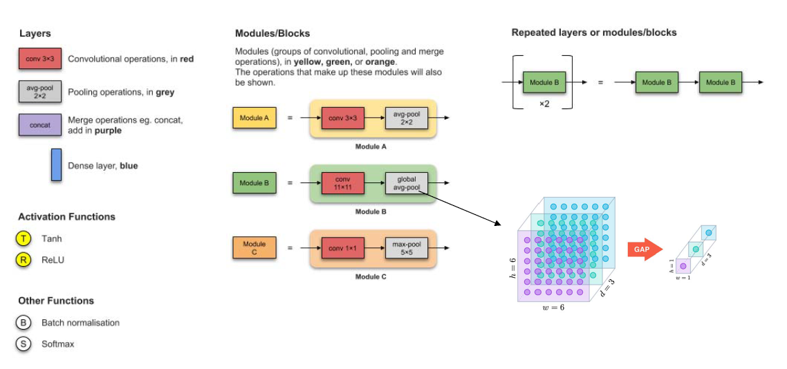
CNNs Variants
Legends
LeNet 5 (1998)
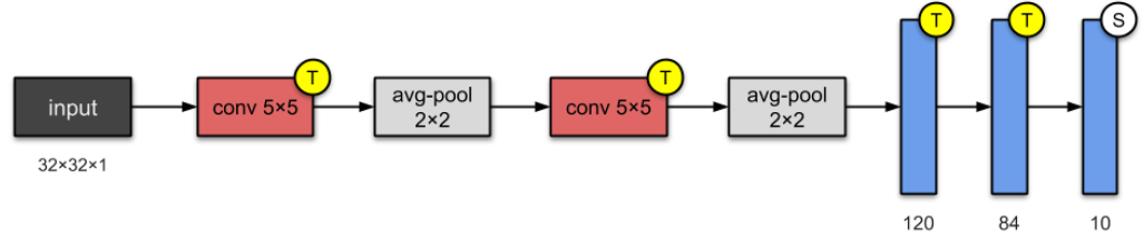
- This architecture has become the standard
- Stacking ConvNet and pooling
- ending network with one or more fc.
AlexNet(2012)
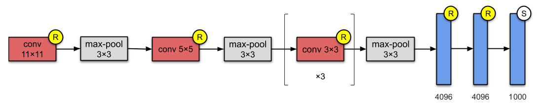
- Apply RelU, pooling, data augmentation, dropout, Xavier initialization
VGGNet - 16 (2014)
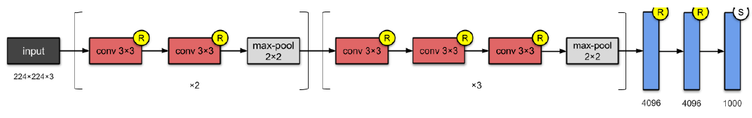
- use only 3x3 sized filter.
- Before VGGNet, they use large filter. But 3x3 sized filter can result same output if use mulitple filter compared with large sized filter.
Effects of 3x3 sized filter
- Decrease number of weights
- If we have an input which has size [50x50x3] and 5x5 sized filter, # of weight is 5x5x3 = 75
- If 3x3 sized filter, # of weight is (3x3x3)+(3x3x1) = 27 + 9 = 36
- 2 consecutive 3x3 filters are same as 5x5 filter
- Increase non-linearity
- Each convolution has ReLU. 3x3 sized filter model has more non-linear function like ReLU than large sized filter model.
GoogleNet Inception-V1 (2014)
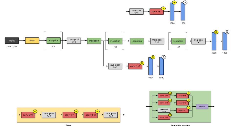
22 layers and 5 Million weights in total
GoogleNet contains Inception Module that has parallel towers of convolutions with different filters, followed by concatenation, which captures different features at 1x1, 3x3 and 5x5.
- In Inception Module, use 1x1 filter before 5x5 filter or 3x3 filter because if we don't use 1x1 sized filter, will get too many weights!
We call 1x1 filter "bottleneck structure".
- 1x1 convolutions are used for dimensionality reduction to remove computational bottlenecks
- 1x1 convolutions add nonlinearity within a convolution
Auxiliary classifier
- Deeper network layers, higher likelihood of vanishing gradient.
- Encourage discrimination in the lower stages
- It only uses in training time.
ResNet-50 (2015)
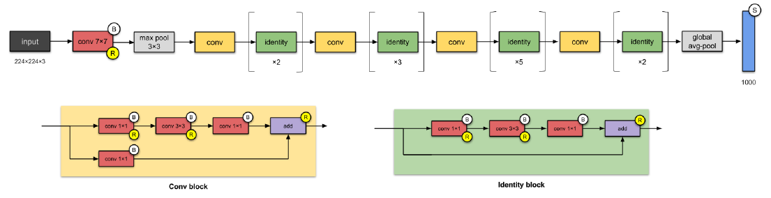
- Skip connections/identity mapping can make deep network
- use batch normalization
- Remove FC layer and replace with GAP(Global Average Pooling)
Motivation
- When networks go deeper, a degradation problem has been exposed.
- 56-layer's result is worse than 20-layer
- But deep layer model has good results in many times.
- So, need some techniques to make deep-layer model
Why ResNet works?
use identity mappings to approximate "shallow network"
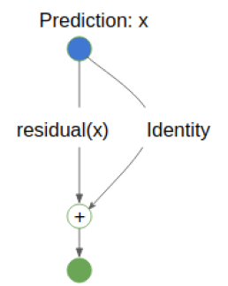
Advantages of Skip Connection
- Reduce optimization difficulty of deeper networks
- Alleviate gradient vanishing problem
- Reuse lower level feature
Xception (2016)
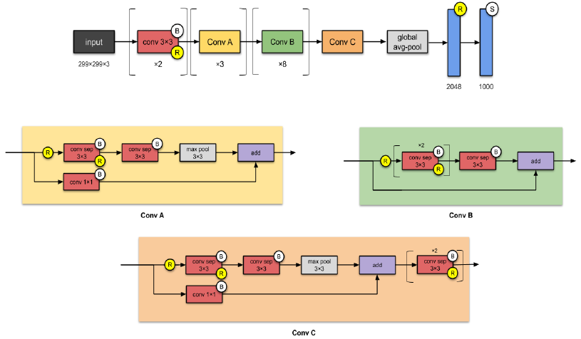
- An adaptation from Inception where the Inception modules have been replaced with depthwise separable convolution(DS-convolution layers)
- Xception has same number of parameters as Inception
Inception - ResNet-V2 (2016)

- Converting Inception modules to Residual Inception blocks
ResNext-50 (2017)
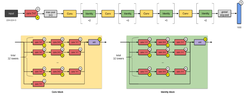
- Adding of parallel towers/branches/paths within each module.
DenseNet (2017)
- Dense blocks where each layer is connected to every other layer in feedforward fashion
- Alleviates vanishing gradient
Squeeze and Extraction - SENet (2017)
- Squeeze and Extraction can do feature recalibration to feature maps from origin networks.
- It is not a complete network, but a wrapper. Thus, we can use it with ResNet, ResNext, Inception etc.
- Improve channel interdependencies at almost no computational cost.
Squeeze
- Get a global understanding of each channel by squeezing the feature maps to a single numeric value.
- use GAP(Global Average Pooling)
Extraction
- Feature Recalibration to computer channel-wise dependencies.
- using Fully connected layer and non-linear function.
'Lecture Note > DeepLearning' 카테고리의 다른 글
| Lecture 2. Network Implementation (0) | 2021.06.16 |
|---|---|
| Lecture1. MLP and Backpropagation (0) | 2021.06.09 |